Analyzing 40+ years of WPR's Chapter a Day show

WPR’s “Chapter a Day” show consists of a book read aloud daily over the radio. I came across it while driving nearly a year ago, and spent some time listening to Truck: A Love Story, chapter 5. I was intrigued and followed up online.

From the WPR webpage:

Started in 1931, “Chapter a Day” is WPR’s longest-running program. Jim Fleming, Norman Gilliland, Michele Good, Melvin Hinton, Baron Kelly and Susan Sweeney read a chapter from a book for a half hour each weekday. Genres are predominately contemporary and range from works of fiction, history and biography.

Impressively, they keep up a comprehensive and well-formatted dataset about all the books they have read since 1983.

It contains

• book title
• book cover image
• author
• publisher
• published year
• ISBN
• description
• whether the book is in public domain
• theme music for the show
• voice actor that read the book
• date range of the book’s reading.

Kudos to the team that maintains this. Note again that while the show started in the 1930s, the dataset only begins in 1983 - so visualized numbers here certainly undercount the show’s entire run.

Such a nicely formatted dataset demands visualizations. So check out a few I made!

This served as a bit of a test for me, as I grapple with how to explore, validate, analyze and present data with LLMs. Claude wrote all code associated with this project, from parsing the data, downloading associated cover images, enriching the data from Google Books and Wikidata, and the data visualizations. I then became the design judgement person, whatever that means, validating the data, deciding what was worth showing, and telling the story.

A lot of posts I see online argue that now that “coding is solved” (not just the AI hype posts), taste is all that matters. So this post is largely the before and after: what AI generated, and how I iterated on it to produce the final result.

I used Opus 5.5 on medium reasoning. I have the monthly subscription, but cost estimate is $84 in API rates. I completed the project over about 4 days in 217 messages.

1. Introducing the topic

Before After

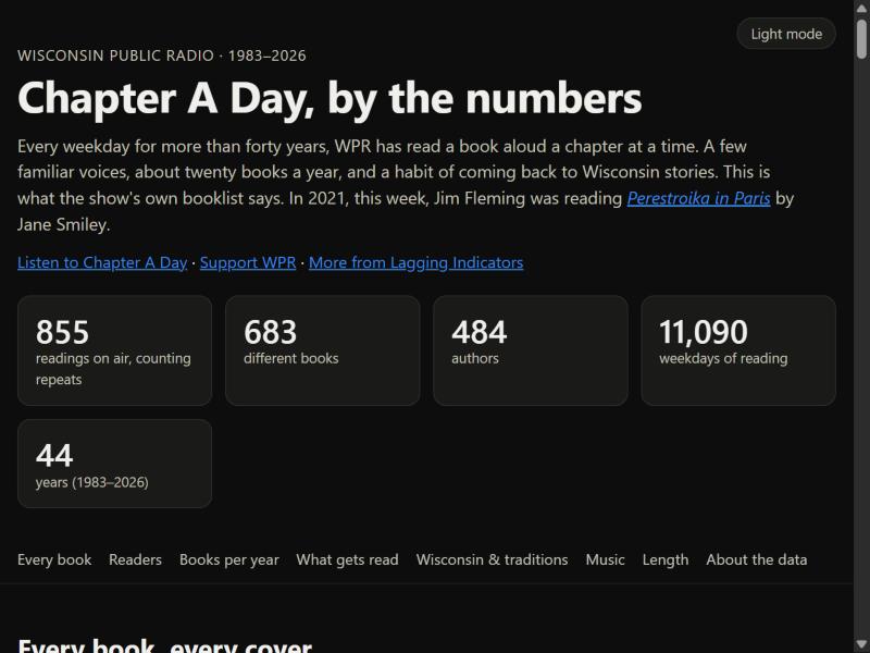
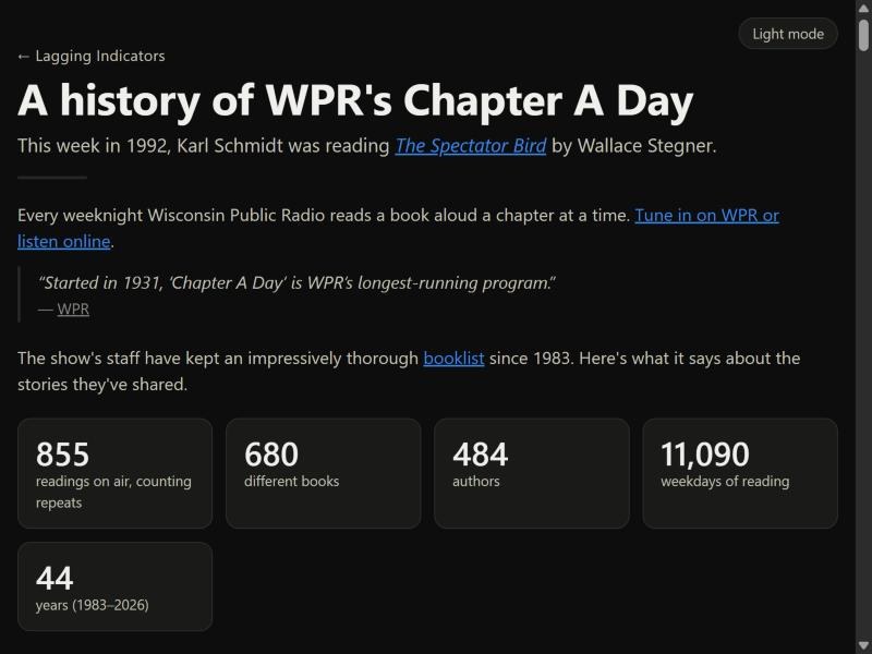
The introduction largely didn’t change. I dropped the Wisconsin Public Radio credit, instead linking to WPR as the source in the opening text and adding the support link at the end, though the screenshot doesn’t show it. I did add the historical reading section at the top, which wasn’t initially included.

I considered putting it at the bottom as a sort of action item, since I think the book discovery is the most interesting part of this as well. But I like that it updates dynamically and picks a random year essentially every time someone loads the page.

2. The readers chart

Before After

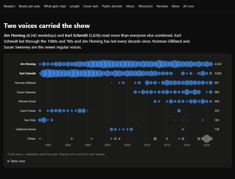
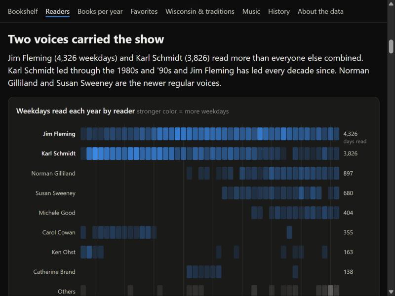
Initially I had envisioned a line chart over time, with little bubbles with the names of the readers. I had previously done this for a team meeting as a fun way to see how our team contributed product tickets over time, and each bubble attached to the line contained our photos.

But in this case, a) many lines just would be flat for a majority, leading to a dull chart, and b) the LLM interpreted this as a bubble per year. But while bubbles overlap, years tend not to, so the shape didn’t match to the phenomenon I was describing.

The strip plot better describes activity per year, even if it doesn’t necessarily demonstrate scale between each reader as well.

Separately, the table view breaks out the “Others” section at the bottom.

On phones:

Before After

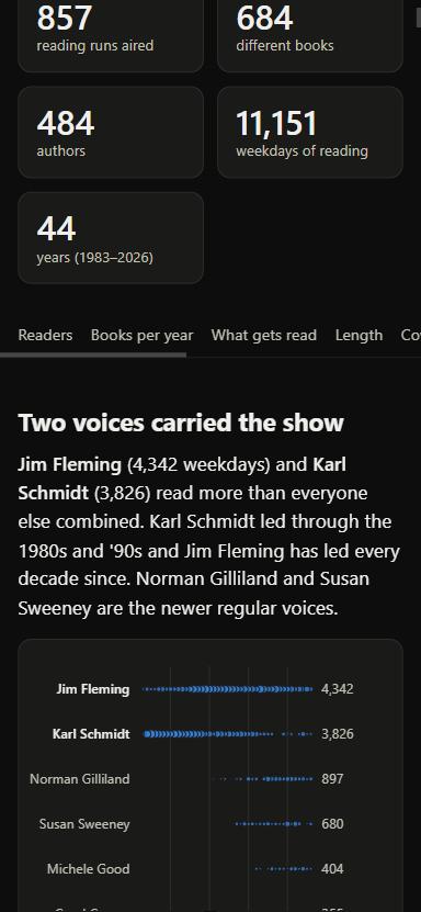
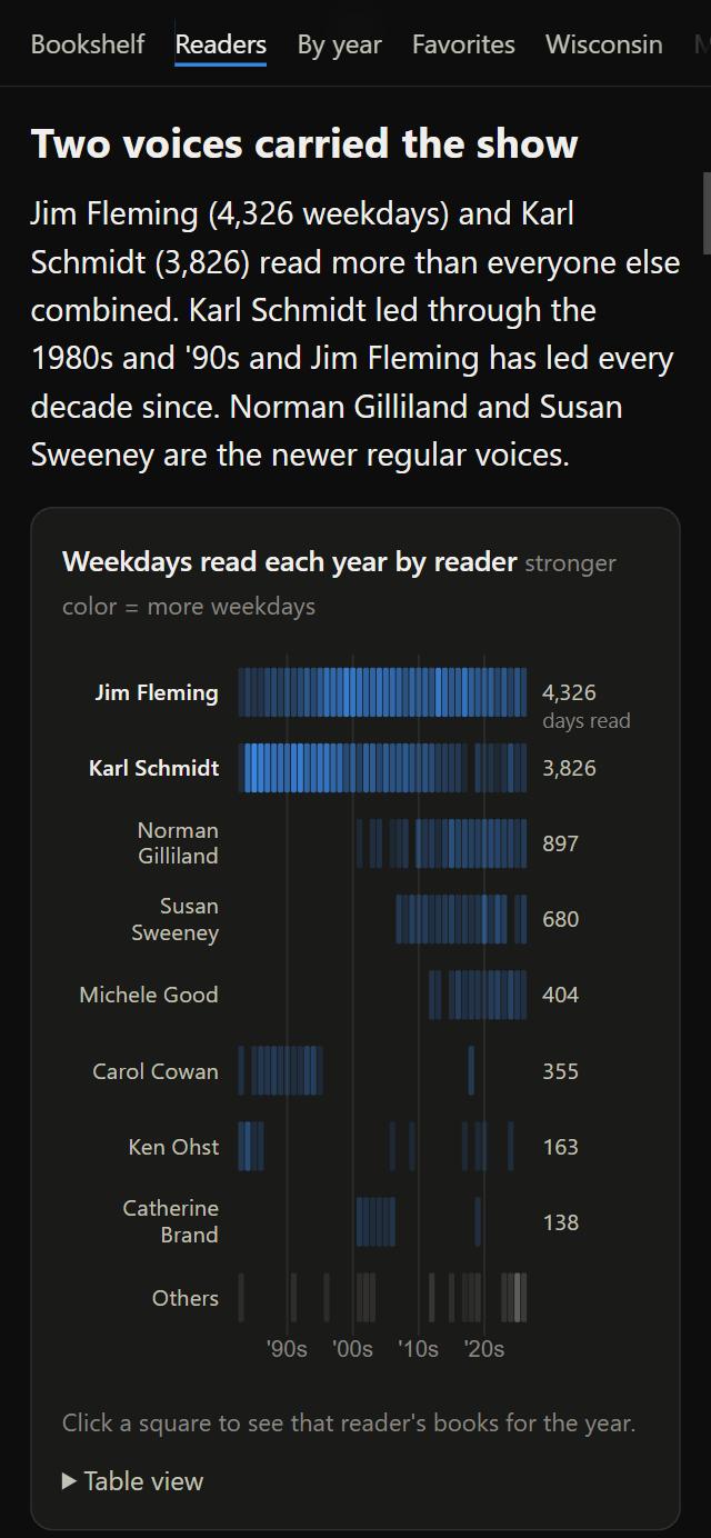
With mobile screens, the clicking to see books each year though is not really possible, if you want a specific year. So I added small buttons on this chart’s modals to change the year to compensate, which makes it simpler to navigate.

The labels on each side I think help balance the chart out + placing the ‘days read’ label at the chart top, rather than the bottom axis, works better for phone users, as we scroll from top to bottom.

The x-axis labels also adjust to shorter decades labels that originally ran together. Unsurprisingly, even Claude struggles with responsive label sizing. I also encountered a bug where tapping the modal and closing it kept the hover label open.

3. About twenty books a year

Before After

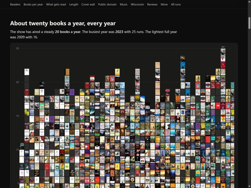
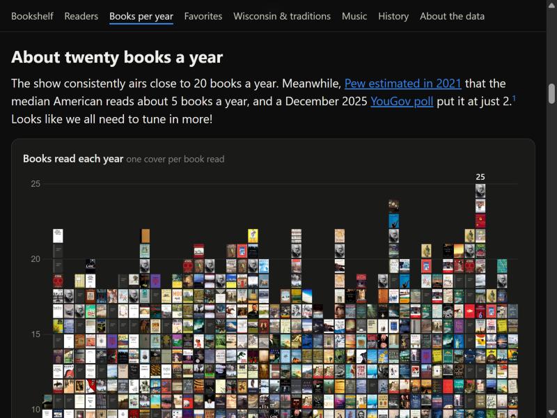
I think one danger in a data set like this is simply adding numbers because they can be calculated, which I think LLMs like to do too. Instead, incorporating the average number of books people read each year provides a better comparison. I also added a footnote indicating that audiobooks are included in this data. I think that’s just my reaction to reading too many blog comments where people challenge whether audiobooks really count as reading.

Additionally, on the live version, if you look closely, you’ll notice that missing covers actually have a slight visual faux spine that I added. Because the covers are so small, it’s a bit tricky, since any text isn’t readable. But a small, lighter line on the left side emulates a cover and helps it blend in better.

4. The bookshelf and the book pop-up

Before After

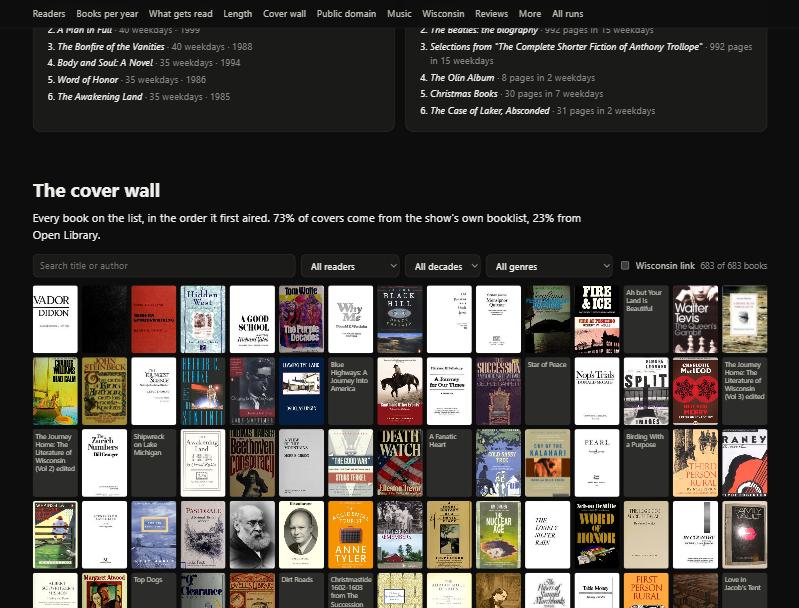
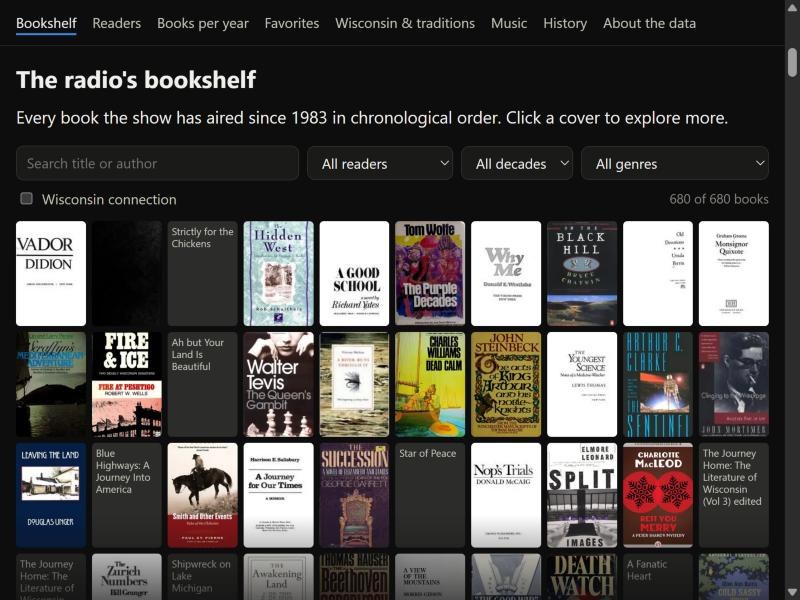
There are small changes here, just to limit the number of books shown and to add a “clear filters” button when a user adjusts a filter. I always find that pretty convenient. I also had to adjust the entries whose covers couldn’t be found, adding in the subtitle on the book page.

Before After

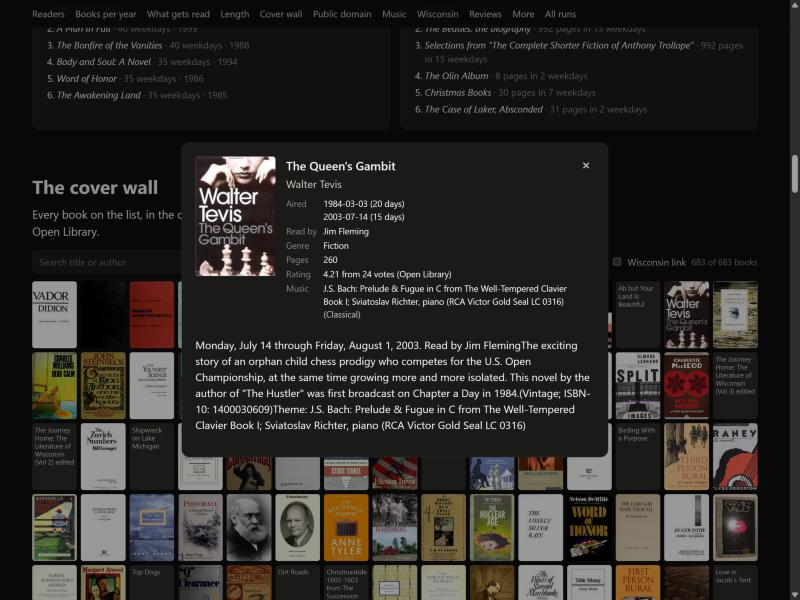
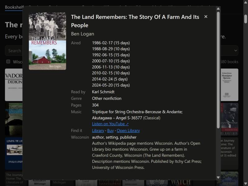
Adding the links to external sites contributes to the idea of the data visualizations being ways to explore and connect to the books, which I like.

The music is a bit tough because it’s manually entered in the data. Rather than trying to link to a specific soundtrack or composer, or cleaning the data like the LLM wanted to do (it just kept trying to prep it better), this links directly to YouTube’s search function, which I think is more straightforward.

There was a problem with WorldCat too: it now essentially forces a user to log in to search. So I switched to just Overdrive, Open Library, and Bookshop.org where available. Neatly, the Wisconsin Public Library Overdrive site allows people to search without logging in, but the collection is less thorough.

One improvement to the data pipeline would be an API that checked if books existed on each site, then direct to the profiles, but finding books is difficult at best, as anyone who has ever cataloged their home library could tell you (me. I recommend the MyLibrary app, but it is still a pain sometimes).

Other than that, just a simple fix to ensure missing covers had a placeholder.

5. Wisconsin-based literature

Bars Maps

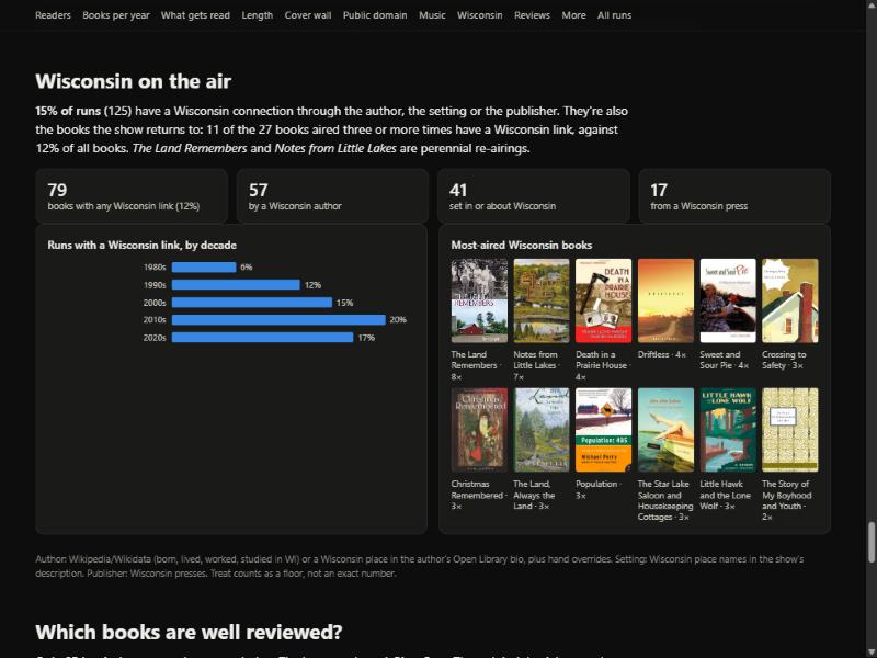
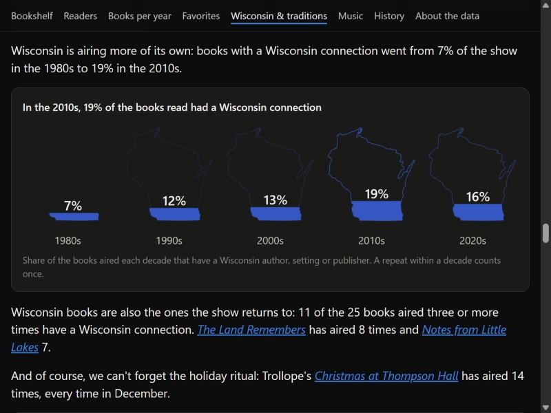
The Wisconsin maps were probably the trickiest to think through. I considered dropping the summary card numbers, but I ended up making them clickable instead, to present a filtered view of the books. You’ll notice that throughout the entire page I tried to keep this sort of functionality: if you click on a bar, for example, it should show you a filtered view of those books. Again, this emphasizes that you can find the books through the visualizations, rather than the number itself being the interesting part.

Truthfully, I’m still mixed about this visualization of Wisconsin, but I did want to do something more distinctive that’s related to the state. The blue is meant to be closer to the state blue on the flag, and you’ll notice the outline increases in opacity as more Wisconsin books get read, repeating the idea of Wisconsin coming into view more strongly. It also uses each decade. Notably, the fill is still an area fill. The numbers inside do bleed out, but that keeps the text large enough to be readable, and I think that’s the right decision. I think it’s a visualization that at least makes people pause for a moment, in a positive way(?).

Originally, for the repeated books, the LLM just put an orange outline around the Wisconsin-connection books within all the repeats, and that played really poorly and was hard to read. It also seemed strange to either separate the Wisconsin repeats from the general repeats (putting those in a bar chart instead) or keep them together. So this just uses the same card with subheaders, which I think is a little neater.

I had to pay additional attention to the sizing of the covers. This is almost the largest book size, matching the top of the bookshelf, because the other three visualizations with covers have to be much smaller so they don’t take up so much of the screen. But I think the covers are much more fun, and again, they draw attention to the books.

6. From a length chart to the history ending

Histogram (generated) Dot plot (try 2) Every week (final)

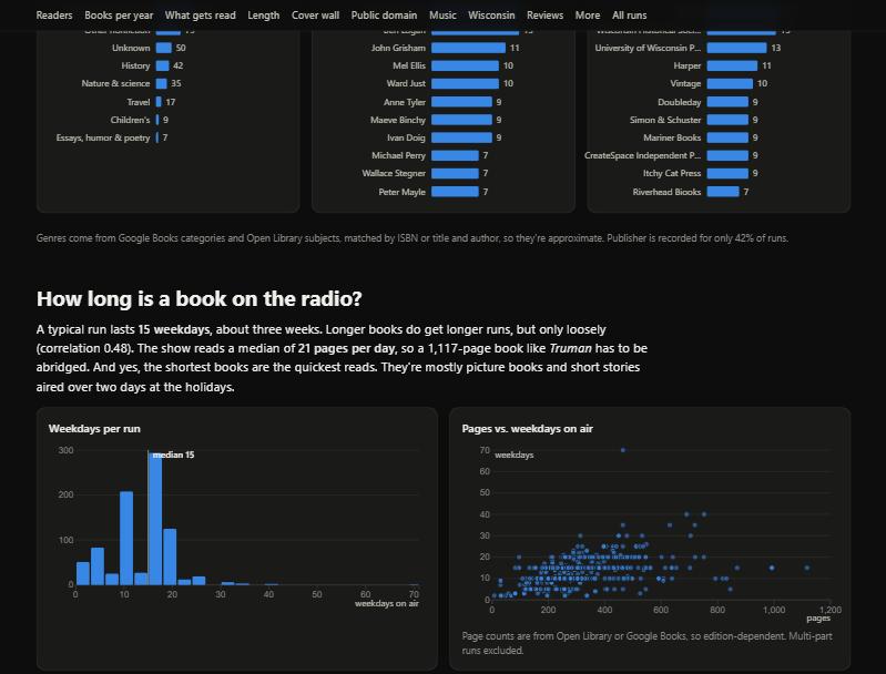
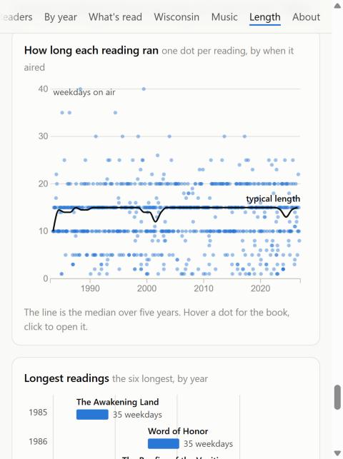
I initially thought how long a book ran would be more interesting. But it was not. Dot charts become less pretty with these flat clusters; it becomes clear that they intentionally choose consistent week-long runs where possible, with these long horizontal dot lines.

So the story became that over time, they are reading longer books less, into a chart I quite like.

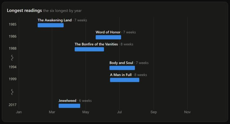
Again, the chart calls out books, rather than hides them in aggregates, and leverages this calendar-esque view. Of course they are clickable.

I think there is some water in the argument bucket that the y-axis year labels should be spaced out properly, but this just creates long gaps of empty space. So the rows stay close together, with a little extra room and a squiggle at the big jumps in years. I also considered re-using the decades labeling, rather than the year callouts too.

The lengths started out in weekdays, but 40 weekdays is not a common timespan, so they are in weeks now. I tried months, but “Just under 1 1/2 months” was still clunky. On small screens, the light gray weeks callout also shifts to the row below, giving more room to the titles too.

The “Color by” modes:

Genre Wisconsin Seasonal

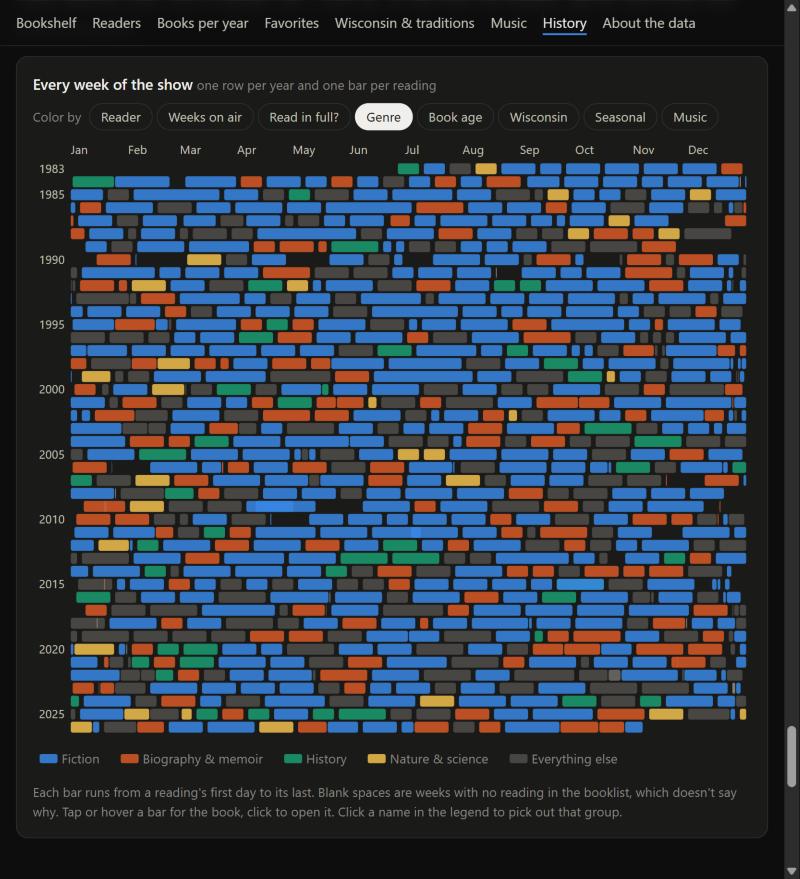
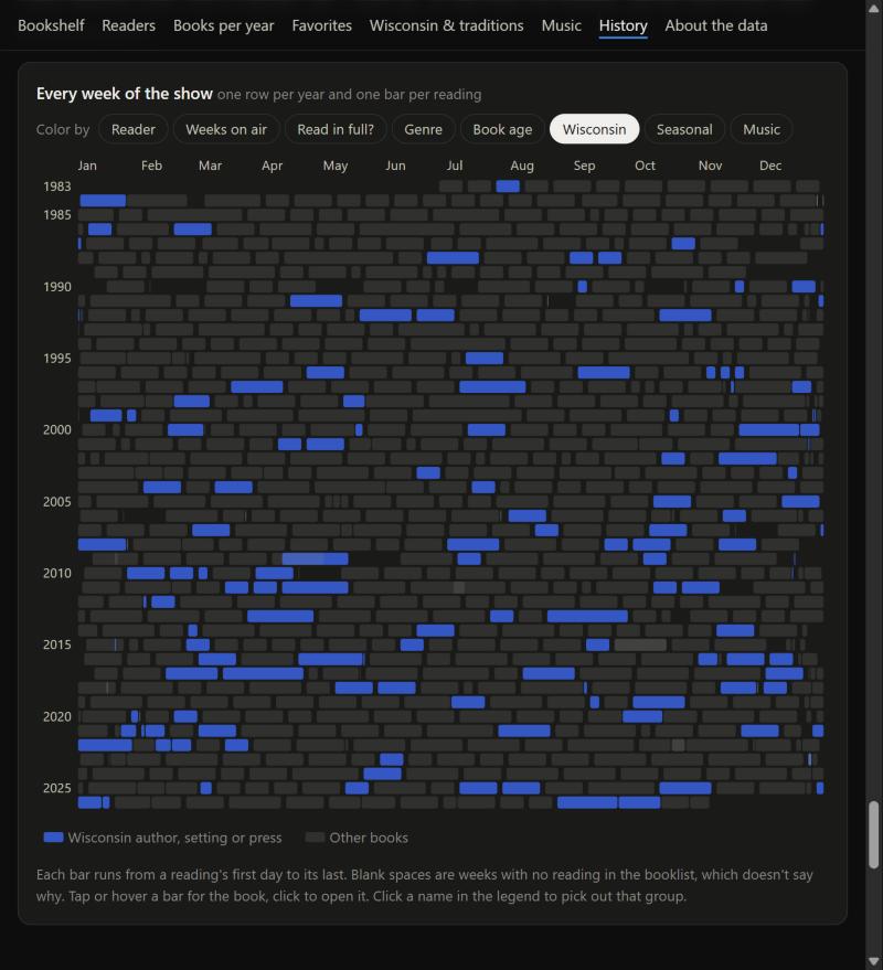
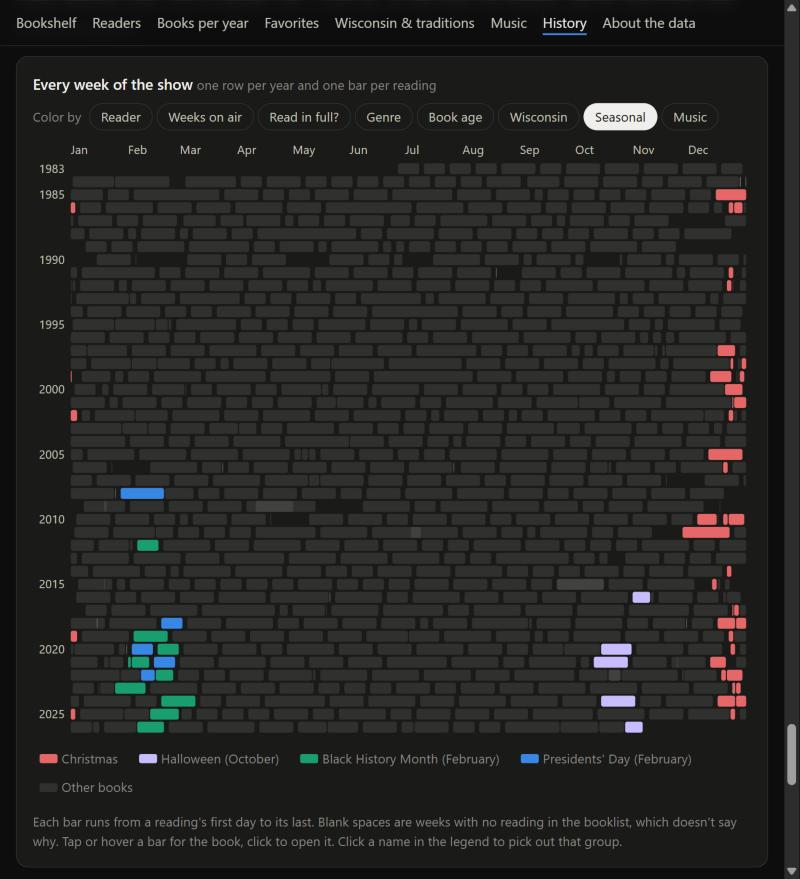
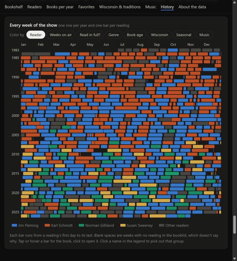
The ending chart tries to tie in all the sections, and I think it strikes a good balance between a comprehensive summary and interactivity. Notably, there aren’t too many patterns, though, so it did take some editing: “Holidays” became “seasonal,” for example, and “length” became “weeks on air.”

On accessibility, the LLM was extremely helpful here after just a brief prompt to validate the accessibility of the page, and it suggested the idea of clicking the legend to highlight each section, which was nice. It also makes implementing these types of changes trivial.

7. Music

Before After

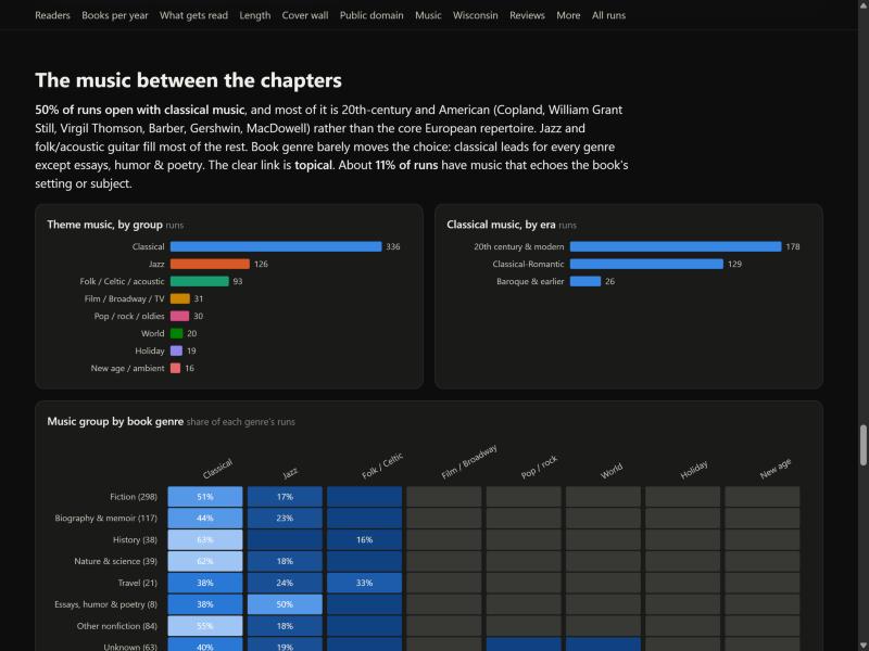
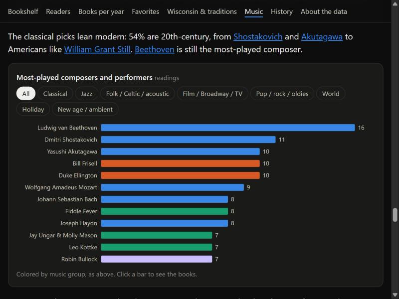
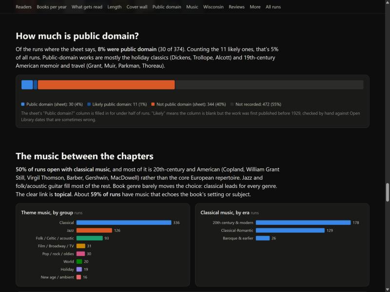
This was another tough one. The music is largely just classical, so the music-grouped-by-book-genre chart just didn’t work, and three charts was too many. I think simplifying it was the right choice. I cut it down to just the top composers per category and added filters, so you can still see the top composers in even the less-played categories. And of course, you can click on a bar to see all the books each composer was associated with.

I think the list of books where the music echoes the book is quite nice, because it kind of connects everything together. Including the covers here adds a bit of personality to a simple list.

8. Cut charts

Ratings Public domain

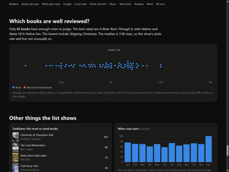
I would have quite liked to keep the well-reviewed books, but there just wasn’t enough data I could pull from, so I cut it. It would be a pretty interesting chart, though, and I would have kept it if I could have built a reliable pipeline. From the few reviews I could get, it looked like an interesting spread.

Overall

It’s probably true to say that writing code to produce data visualizations, even complex ones, won’t be that common anymore, especially because so many data visualizations are one-off.

But I also think we can now say that the standard we expect from a data visualization is just perfect. I don’t know if there’s a defense for not having accessible, interactive, high quality data visualizations. We can easily iterate on a chart until the labels align perfectly and it adheres to the designer’s taste.

I am deeply curious about how LLM-driven data pipelines will progress. Claude was able to convert, prepare, and enrich this dataset extremely quickly, for example. Validating the data connections worked took me more time than it took Claude to write a Google Books API script. But I think many users will not want to take the time to make sure it’s right. People will pay for that validation, because they want to continue building.

Before, I would think “ah this is just a hard chart and a basic one is fine it just needs to communicate the data.” Now it is “did someone bother to pay attention to what they want me to care about?”

Separately, now that people can make these pretty charts, I wonder if this will further standardize how data visualizations look, sort of like how modern websites all cluster along the same design standards and how Datawrapper styles dominate newspapers.

Mockups are now almost instantaneous, and you can experiment so much quicker with how the visual shapes a person’s perception. Will people actually use that ability to really experiment, or will they just accept whatever Claude’s default settings are? Is my opinionated take about how I want something to look and act worth anything? Is my taste distinctive enough?